Negative binomial DE with quasi-likelihood dispersion shrinkage
delnx implements GPU-accelerated negative binomial GLMs following the glmGamPoi approach with quasi-likelihood dispersion shrinkage for differential expression analysis. The two-step workflow (nb_fit + nb_test) separates model fitting from hypothesis testing, allowing you to reuse a single fit across multiple contrasts.
import delnx as dx
import scanpy as sc
import numpy as np
import matplotlib.pyplot as plt

# Load example pseudobulk data
adata = sc.read_h5ad("data/GLI3_KO_45d_pseudobulk.h5ad")
adata.obs["GLI3_KO"] = adata.obs["GLI3_KO"].astype(str)  # Ensure string type for design matrix

# Use raw counts (X contains normalized values)
adata.X = np.round(np.asarray(adata.layers["counts"])).astype(np.float64)

print(adata)
print(f"Count range: {adata.X.min():.0f} - {adata.X.max():.0f}")
AnnData object with n_obs × n_vars = 28 × 16199
    obs: 'psbulk_replicate', 'cell_type', 'organoid', 'GLI3_KO', 'psbulk_cells', 'psbulk_counts', 'size_factor'
    var: 'dispersion', 'dispersion_deseq', 'dispersion_mle', 'dispersion_edger', 'mean', 'mean_norm'
    uns: 'log1p'
    layers: 'counts', 'psbulk_props'
Count range: 0 - 123900
Fit the model
nb_fit handles everything in one call: size factor estimation, dispersion MLE with Cox-Reid bias adjustment, quasi-likelihood shrinkage, and coefficient fitting via IRLS.
# Fit negative binomial GLMs with quasi-likelihood dispersion shrinkage
fit = dx.tl.nb_fit(adata, condition_key="GLI3_KO", reference="True")

print(f"Coefficients: {fit.design_column_names}")
print(f"Genes fitted: {len(fit.overdispersions)}")
print(f"Dispersion range: {fit.overdispersions.min():.4f} - {fit.overdispersions.max():.2f}")
INFO     Fitting 16199 genes with 2 coefficient(s)
INFO     Applying quasi-likelihood shrinkage
Coefficients: ['Intercept', 'GLI3_KO[T.False]']
Genes fitted: 16199
Dispersion range: nan - nan
fig, axes = plt.subplots(1, 2, figsize=(14, 5))

# Left: dispersion distribution
valid_disp = fit.overdispersions[fit.overdispersions > 0]
axes[0].hist(np.log10(valid_disp), bins=50, color="steelblue", alpha=0.7, edgecolor="white")
axes[0].set_xlabel("log10(dispersion)")
axes[0].set_ylabel("Number of genes")
axes[0].set_title("Dispersion distribution")
axes[0].axvline(np.log10(np.median(valid_disp)), color="red", linestyle="--", label=f"median={np.median(valid_disp):.3f}")
axes[0].legend()

# Right: mean-dispersion relationship
gene_means = np.asarray(adata.X).mean(axis=0) if hasattr(adata.X, 'toarray') else adata.X.mean(axis=0)
mask = (gene_means > 0) & (fit.overdispersions > 0)
axes[1].scatter(np.log10(gene_means[mask]), np.log10(fit.overdispersions[mask]), s=5, alpha=0.3)
axes[1].set_xlabel("log10(mean expression)")
axes[1].set_ylabel("log10(dispersion)")
axes[1].set_title("Mean-dispersion relationship")

plt.tight_layout()
plt.show()
plt.close()
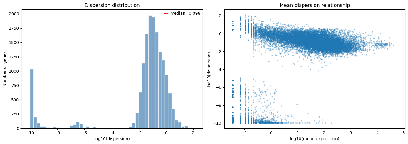
The left panel shows the distribution of MLE dispersions across genes. Most genes cluster around the median, with a long tail of highly variable genes.
The right panel shows the characteristic mean-dispersion relationship: lowly expressed genes tend to have higher dispersion, while highly expressed genes converge toward lower dispersion values.
Test for differential expression
Now we test for DE using the fitted model. nb_test uses a quasi-likelihood F-test, which accounts for the uncertainty in dispersion estimation.
# Test for differential expression
de_results = dx.tl.nb_test(adata, fit, contrast="GLI3_KO[T.False]")

print(de_results)
      feature    log2fc      coef       stat          pval      padj
0        EMX1  6.761568  4.686762  83.710401  4.326881e-10  0.000007
1      ZNF429 -5.335782 -3.698482  75.925150  1.246159e-09  0.000010
2       SFTA3 -8.920224 -6.183028  60.244111  1.368526e-08  0.000074
3       CXXC4 -0.873021 -0.605132  54.949587  3.389955e-08  0.000106
4        ZIC5  1.904016  1.319763  54.774321  3.496747e-08  0.000106
...       ...       ...       ...        ...           ...       ...
16194    GJB3       NaN       NaN        NaN           NaN  1.000000
16195   CCL16       NaN       NaN        NaN           NaN  1.000000
16196    CCR1       NaN       NaN        NaN           NaN  1.000000
16197   PLET1       NaN       NaN        NaN           NaN  1.000000
16198    ORM2       NaN       NaN        NaN           NaN  1.000000

[16199 rows x 6 columns]
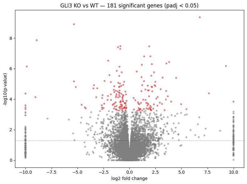
# Volcano plot
fig, ax = plt.subplots(figsize=(8, 6))

sig = de_results["padj"] < 0.05
colors = np.where(sig, "tab:red", "tab:grey")

ax.scatter(de_results["log2fc"], -np.log10(de_results["pval"]), c=colors, s=10, alpha=0.5)
ax.axhline(-np.log10(0.05), color="black", linestyle="--", linewidth=0.5, alpha=0.5)
ax.set_xlabel("log2 fold change")
ax.set_ylabel("-log10(p-value)")
ax.set_title(f"GLI3 KO vs WT — {sig.sum()} significant genes (padj < 0.05)")

plt.tight_layout()
plt.show()
plt.close()